Control Theory Quick Reference

The study of many kinds of systems, control policies, matrices, and vector spaces (including functions) comprises control theory. This document is a free, community-driven growing dictionary of these terms, designed for quickly finding more information about them, rather than hunting down definitions online or in a textbook.

Contributions are not just welcome, they are necessary to keep this project going strong. If you find potential for this project to help someone else, please consider generously donating 15 minutes of your time to describe one term that might confuses someone else, refine an inaccurate/incorrect definition, or fix that one design issue that bothers you. Little contributions like these will add up to make a lasting impact on control theory studies.




Variables and Symbols


x	state vector (state space) (W) Type: Rⁿ



H	Hamiltonian matrix Hamiltonian (Hamiltonian mechanics) (W) type: Rⁿ →R Assuming discrete time linear system: $T Hk = L (xk,uk,k)+ pk+ 1f(xk,uk,k)$



ℒ	the Lagrangian type: Rⁿ →R



B	A ball, defined as ${ n } B (x0,𝜖) = x ∈ R :∥x− x0∥ ≤ 𝜖$



C	C¹ = Continuously differentiable, i.e. the first derivative is continuous. Cⁿ = The n^th derivative is continuous. C: the set of all complex numbers a+ bi where a and b are real and i =



e_#	The #th unit vector $(\|) ( ) ( ) \|1\| \| 0\| \|0\| \|\|0\|\| \|\| 1\|\| \|\|0\|\| \|\| \|\| \|\| \|\| \|\| \|\| e1 = \|\|0\|\| , e2 = \|\| 0\|\| , e3 = \|\|1\|\| , ... \|\| ...\|\| \|\| ...\|\| \|\| ...\|\| ( ) ( ) ( ) 0 0 0$



∇	The del operator, which represents one of many long but similar operators on a vector field v ∈Rⁿ. ∇f: Gradient of a function f : Rⁿ →R, returning an n-dimensional vector. (W) This vector points in the direction of the greatest increase, and its magnitude is the slope. For example, a mountain climber could approximate the shape of a convex mountain as a function f_mountain that computes the altitude given some latitude and longitude (assuming a very small mountain very far from the poles). In other words, f_mountain : R² →R. The climber could know which direction to climb to summit the peak: it’s the direction ∇f, and the grade or slope of the mountain is Note that if n = 1, ∇f is the standard derivative of f. Formally speaking: $n ∂f ∇f = ∑ ---ei i=1∂xi$ ∇⋅v: The divergence of a vector field v ∇×v: The curl of a vector field v Δf: the Laplace operator on a function f : Rⁿ →R, equivalent to the divergence of the gradient of f, i.e. $δf = ∇ 2f = ∇ ⋅∇f$



J	Cost to go function type: Rⁿ →R



p	Lagrange multiplier (W)



	Lie bracket notation (W) = b^Ta



	Vector norm (TODO) Matrix norm (TODO) Functional norm (TODO) Norm of a system y(u, t) = h(u(t)), where y is an n-dimensional the output of the system, u is an m-dimensional control vector (TODO)

Named Theorems and Conditions

Poincaré-Bendixson theorem

TODO

Small-gain Theorem

Given

H₁: an Input-Output System with input e₁ and output y₁ that is finite-gain ℒ_p-stable
H₂: an Input-Output System with input e₂ and output y₂ that is finite-gain ℒ_p-stable
y₁ = H₁e₁
y₂ = H₂e₂
e₁ = u₁ −y₂
e₂ = u₂ −y₁

By the definition of finite-gain ℒ_p-stable,

∥∥y ∥∥ ≤ γ ∥e ∥ + β 1τ ℒp 1 1τ ℒp 1

(The ℒ_p norm of the y₁ is truncated by τ, i.e. the system response is zero when t > τ. This is less than or equal to The ℒ_p norm of the e₁ truncated by t < τ, multiplied by some gain value γ₁, plus some bias β₁)

As long as a system does not have a finite escape time, we can compute the ℒ_p norm of the system.

Likewise,

∥ ∥ ∥y 2τ∥ℒp ≤ γ2∥e2τ∥ℒp + β2

The Small-gain Theorem tells us,

∥∥###∥∥ ( ) ( ) ∥∥y1τ∥∥ ≤ ----1--- ∥u1τ∥ + γ 2∥u2τ∥ + γ2β1+ β2 = γ3 some ℒp-stable system ∥∥y2τ∥∥ 1 − γ1γ2 ℒp ℒp ℒp

(1)

Therefore, if γ₁ and γ₂ are less than one, the feedback connection is input/output stable (finite-gain ℒ_p-stable)

Terms

Classes of Systems

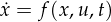
Given a dynamic system

Dynamic system
$x˙= f(x,u,t)$
Time-invariant system is a dynamic system
$˙x = f(x ,u)$
Autonomous system is a dynamic system
$˙x = f(x,t)$
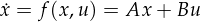
Linear system (W) is a dynamic system
$˙x = f(x ,u,t) = A (t)x + B(t)u$
Linear time-invariant system is a linear system and a time-invariant system
$˙x = f(x,u) = Ax + Bu$

Lipschitz Continuity (W,) (UC Berkley)

Lipschitz continuous functions are continuous and differentiable almost anywhere in a domain.

Given a domain D and a function f : D →R, D ∈Rⁿ,
f is Lipschitz continuous if ∃L > 0 such that |f(x) −f(y)| < L||(x−y)||∀x, y ∈ D

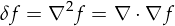
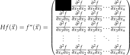
Hessian (W), (Kahn Academy), (Wolfram)

A n x n matrix of all 2nd order partial derivatives of some function f : Rⁿ →R

$(#-∂2f---∂2f--∂2f- -∂2f-) |#∂x12∂x1∂x12∂x2∂x12∂x3...∂x12∂xn| || ∂x∂f∂x-∂x∂f∂x-∂∂x-f∂x-...∂x∂f∂x-|| || -2∂2f1--2∂2f2-∂22f3 -2∂2fn|| Hf (⃗x) = f”(⃗x) = || ∂x3∂x1∂x3∂x2∂x3∂x3...∂x3∂xn|| || ... ... ... ... ... || (--∂2f---∂2f--∂2f- --∂2f-) ∂xn∂x1∂xn∂x2∂xn∂x3...∂xn∂xn$ (2)
The determinant of a Hessian matrix

definite (W)

Warning: this definition does not appear to be common outside of controls

Given a real-valued, continuously differentiable function V(x) : R →R
V(x) can be classified as

(globally) positive semidefinite if
$V(x) ≥ 0 ∀x ∈ R$

(v is greater than or equal to 0 regardless of x)
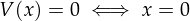
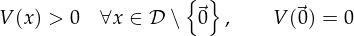
(globally) positive definite if positive semidefinite AND
$V (x) = 0 ⇐ ⇒ x = 0$

(V(x) is zero if and only if x is zero)
(globally) negative semidefinite if
$V(x) ≤ 0 ∀x ∈ R$

(v is less than or equal to 0 regardless of x)
(globally) negative definite if negative semidefinite AND
$V (x) = 0 ⇐ ⇒ x = 0$

(V(x) is zero if and only if x is zero)
locally positive definite (l.p.d) if
$V(x) ≥ 0 ∀x ∈ N$
where N is a small open neighborhood containing 0

(v is greater than or equal to 0 regardless of x in some small open neighborhood N that contains the zero vector)

AND

$\text{[math]}$

(V(x) is zero if and only if x is zero)

Note that the criteria for a function to be locally positive definite are similar, but more relaxed than, those for globally positive definite functions.
positive definite on some domain D ∈Rⁿ if
we only care if the conditions for positive definite functions hold for all x in D.

Stability (MIT)

Given an autonomous system

˙x = f(x,t)

and some open connected region 𝒟 containing 0

Stability is usually used to describe trajectories around the origin of a system.

Stability
The equilibrium point x = 0 is stable if ∀𝜖 > 0, ∃δ(𝜖) > 0 such that < δ < 𝜖
- In the sense of Lyapunov
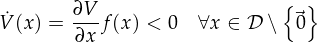
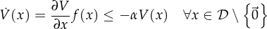
  If there exists a scalar, continuously-differentiable function V(x) such that
  ${ } V(x) > 0 ∀x ∈ 𝒟 ∖ ⃗0 , V(⃗0) = 0$
  
  (V(x) is a locally positive definite function)
  
  AND
  
  ${ } V˙(x) = ∂V-f(x) ≤ 0 ∀x ∈ 𝒟 ∖ ⃗0 , V (⃗0) = 0 ∂x$
  
  (V(x) is a locally negative semidefinite function)
  
  then the origin is stable in the sense of Lyapunov, and V(x) is a Lyapunov function of f(x).
Instability
The equilibrium point x = 0 is unstable if it is not stable
Asymptotic stability
The equilibrium point x = 0 is asymptotically stable if it is stable and ∃δ₁ such that < δ₁ lim _t→∞x(t) = 0
- In the sense of Lyapunov
  The origin is asymptotically stable in the sense of Lyapunov if stable AND
  $∂V { } V˙(x) =---f(x) < 0 ∀x ∈ 𝒟 ∖ ⃗0 ∂x$
  
  (V(x) is a locally negative definite function)
Exponential stability
- In the sense of Lyapunov
  The origin is exponentially stable in the sense of Lyapunov if stable AND
  $\text{[math]}$
Uniform stability
The equilibrium point x = 0 is uniformly stable if it is stable and, for each epsilon > 0, there exists a δ(𝜖) > 0, independent of t₀.

Stability (continued)

Global asymptotic stability
- In the sense of Lyapunov
  If the origin is globally asymptotically stable in the sense of Lyapunov if is asymptotically stable and
  $∥x∥ → ∞ =⇒ V(x) → ∞$
  
  (V(x) is radially unbounded)
L-stability
(TODO)
I/O L-stability
(TODO)
Finite-gain L-stability
(TODO)
Small-signal I/O L-stability
(TODO)
Small-signal finite-gain L-stability
(TODO)

Class κ function

A continuous scalar function on R⁺ is

class κ if it is:
- zero at zero
- strictly increasing
- continuous
class κ_∞ if it is:
- zero at zero
- strictly increasing
- continuous
- ∞ at ∞

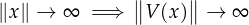
Radially Unbounded function

A function V(x) is radially unbounded if

∥∥ ∥∥ ∥x∥ → ∞ = ⇒ V (x) → ∞

sup (supremum)

Like a maximum of a functions, but includes limits that aren’t necessarily a part of the domain of the function. (TODO)

Hurwitz

Hurwitz (polynomial):
A polynomial whose roots that are all in the left-half plane. (In other words, the real part of every root is strictly negative)
Hurwitz (matrix) (W):
A square matrix whose characteristic polynomial is Hurwitz, meaning all eigenvalues are in the left-half plane. (In other words, the real part of every eigenvalue is strictly negative)
Routh-Hurwitz stability criterion (IEEE):
TODO

Any hyperbolic fixed point (or equilibrium point) of a continuous dynamical system is locally asymptotically stable if and only if the Jacobian of the dynamical system is Hurwitz stable at the fixed point.

A system is stable if its control matrix is a Hurwitz matrix.

The negative real components of the eigenvalues of the matrix represent negative feedback. Similarly, a system is inherently unstable if any of the eigenvalues have positive real components, representing positive feedback.

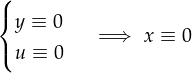
Zero-state observable

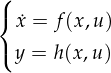
A time-invariant system of the form

( { ˙x = f(x,u) ( y = h(x,u)

is zero-state observable if

( { y ≡ 0 =⇒ x ≡ 0 ( u ≡ 0

In other words, when u = 0, any nonzero state behavior will be observed at the output (y≠0)

Sets

Invariant Set
A set of vectors M is invariant with respect to ẋ = f(x) if
$x(0) ∈ M =⇒ x(t) ∈ M , ∀t ∈ R$

(if a solution belongs to M at some time instant, then it belongs to M for all future and past time)
Positively Invariant Set
A set of vectors M is positively invariant with respect to ẋ = f(x) if
$x(0) ∈ M =⇒ x(t) ∈ M , ∀t ≥ 0$

(if a solution belongs to M at some time instant, then it belongs to M for all future time)
Open Set
A set D ⊂Rⁿ (D, which is a set of real vectors) is an open set if
$∀x ⊂ D, ∃𝜖 > 0 such that B (x ,𝜖) ⊂ D$

(for all vectors x in the domain D, there exists a real scalar 𝜖 such that we can create a ball around x with radius 𝜖, and that whole ball is in D)
Closed Set
A set D ⊂Rⁿ (D, which is a set of real vectors) is a closed set if
$n R ∖D is an open set$

(everywhere outside of D is open)
Bounded Set
A set D ⊂Rⁿ (D, which is a set of real vectors) is a bounded set if
$∃ 𝜖 > 0 such that D ⊂ B(0,𝜖)$

(D fits in a ball with a finite, constant radius 𝜖)
Compact Set
A set D ⊂Rⁿ (D, which is a set of real vectors) is a compact set if it is closed and bounded.

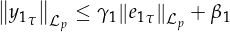
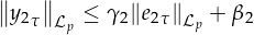
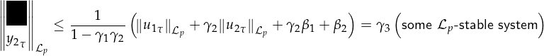
Passivity

For a system y = h(u, t), h : R^m × [0,∞ ) →Rⁿ
(output state y (an n-dimensional vector) is a function of the input state u (an m-dimensional vector) and time t)

Invariant Set
A set of vectors M is invariant with respect to ẋ = f(x) if
$x(0) ∈ M =⇒ x(t) ∈ M , ∀t ∈ R$

(if a solution belongs to M at some time instant, then it belongs to M for all future and past time)

Adjoint

The {adjoint or Hermitian transpose}of a matrix A (Wolfram) is its conjugate transpose, denoted as A′, A^∗, A^H, or A^† i.e.

$H --T A = A$

Interesting properties of ajoint matrices:
- A^H = A^T = A^T
- If a matrix is its own conjugate transpose, that matrix is called self-adjoint or Hermetian
- If A is a real matrix, A^H = A^T
Warning: In some older literature, the ”adjoint of a matrix” may mean the adjunct matrix of a square matrix (W)
The adjoint representation of a vector space (Wolfram)
(TODO)
The adjoint equation (W)
(TODO)